Excel division sounds simple until your spreadsheet decides to be dramatic. One second you are trying to calculate unit price, conversion rate, profit margin, or cost per item. The next second Excel is flashing #DIV/0! at you like it just discovered betrayal. The good news is that dividing two columns in Excel is actually very easy once you know the rhythm. Better still, it only takes four quick steps to set it up properly and copy the formula down your sheet.
Whether you are working with sales totals, inventory counts, ad metrics, classroom grades, or household budgets, knowing how to divide one column by another is one of those tiny Excel skills that saves a surprising amount of time. And once you learn it, you will start using it everywhere. Excel may not have a giant button labeled “Do the math for me, thanks,” but it does give you a clean, reliable formula method that works beautifully.
In this guide, you will learn exactly how to divide two columns in Excel in four quick steps, how to avoid common formula mistakes, how to fix division errors, and how to make your worksheet look like it was built by someone who absolutely knows what they are doing.
Why You Might Need to Divide Two Columns in Excel
Dividing two columns is one of the most common spreadsheet tasks because it turns raw numbers into useful insights. Here are a few everyday examples:
- Price per unit: total cost divided by quantity
- Conversion rate: orders divided by visitors
- Average revenue: revenue divided by number of customers
- Hours per task: total hours divided by total completed items
- Grade percentage: points earned divided by total possible points
In all of these cases, Excel helps you perform the same operation row by row. You enter one formula, copy it down, and suddenly your spreadsheet goes from “pile of numbers” to “actual analysis.” It is the kind of upgrade that makes you feel oddly powerful for someone sitting in sweatpants with coffee stains nearby.
The Basic Idea Behind Excel Division
Before jumping into the steps, here is the simple rule: in Excel, division uses the forward slash /. If you want to divide the value in cell A2 by the value in cell B2, you type:
=A2/B2
That is it. No DIVIDE() function. No hidden button. No secret underground menu. Just an equal sign, a cell reference, a forward slash, and another cell reference.
If you are dividing two entire columns, you usually start in a third column where the result will appear. For example:
- Column A = Total Sales
- Column B = Number of Orders
- Column C = Average Sale Value
In cell C2, you would enter =A2/B2. Then you fill the formula down so each row calculates automatically.
How to Divide Two Columns in Excel in 4 Quick Steps
Step 1: Organize Your Data Clearly
Start by making sure your two columns are lined up correctly. Each row should contain related values. If column A has revenue and column B has units sold, row 2 should represent one matching record, row 3 another, and so on. Excel is smart, but it cannot fix chaos that began as “I pasted everything in a hurry and hoped for the best.”
Here is a simple example:
| Total Revenue | Units Sold | Revenue per Unit |
|---|---|---|
| 250 | 10 | |
| 180 | 6 | |
| 320 | 8 |
Leave the third column empty for the result. Give it a clear header, such as Revenue per Unit, Rate, Ratio, or Average. Naming things well in Excel is not flashy, but it saves future-you from staring at column J and wondering what on earth Calc 2 Final Maybe was supposed to mean.
Step 2: Enter the Division Formula
Click the first result cell. In our example, that is C2. Then type the formula:
=A2/B2
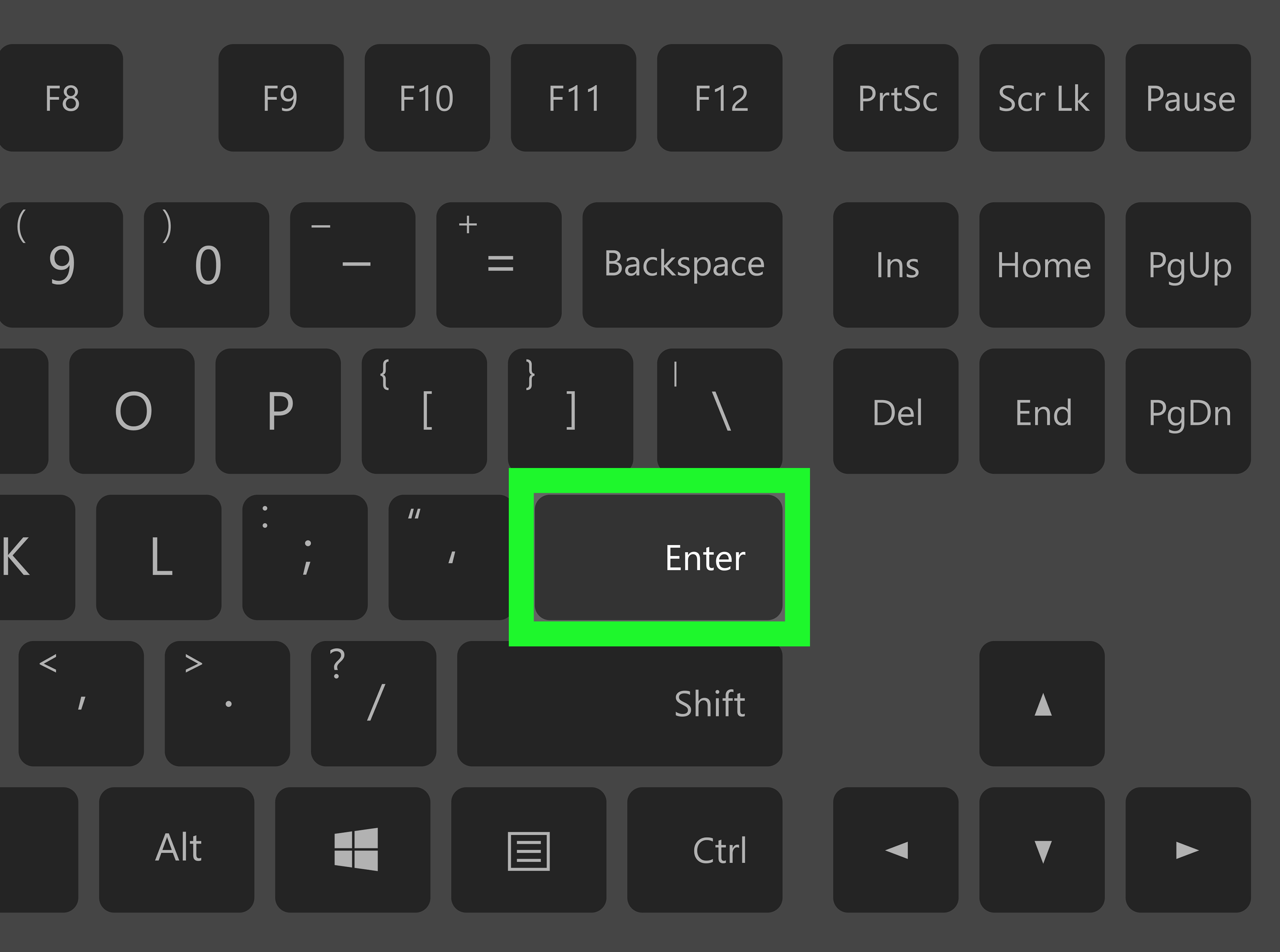
Press Enter. Excel will immediately calculate the result.
Using the sample data above:
250/10becomes 25180/6becomes 30320/8becomes 40
If you prefer clicking instead of typing, you can build the formula this way:
- Type
= - Click cell
A2 - Type
/ - Click cell
B2 - Press Enter
This method is especially useful when your sheet is large and you do not want to mistype cell references. One wrong letter or number in a formula can send you into a 15-minute detective story featuring zoom controls, muttering, and mild regret.
Step 3: Fill the Formula Down the Column
Now that the first row works, you need to apply the same formula to the rest of the rows. The easiest method is the fill handle, which is the small square in the bottom-right corner of the selected cell.
Here is how:
- Select the cell with the formula, such as
C2 - Move your cursor to the bottom-right corner until it becomes a small plus sign
- Drag downward through the rows you want to calculate
Excel will automatically adjust the references for each row:
C2 = A2/B2C3 = A3/B3C4 = A4/B4
You can also double-click the fill handle if the adjacent data column is continuous. That is a great little shortcut when your dataset is long and your mouse hand is already negotiating a peace treaty with your wrist.
Another handy option is Ctrl + D. If you select the formula cell and the empty cells below it, pressing Ctrl + D fills the formula down in one move.
Step 4: Format and Check Your Results
Once the formulas are in place, scan the results column for anything unusual. You might want to format the numbers as:
- General numbers for plain results
- Currency for values like cost per item
- Percentage if the result is a ratio you want displayed as percent
- Number with decimal places for cleaner presentation
To format the column, select it and choose the number style from the Home tab. If your results look overly long, reduce the decimals to two places. Unless you are doing scientific work, nobody needs to admire thirteen decimal places in a cost-per-click calculation.
This final step matters because a correct formula with bad formatting can still look confusing. Excel has a talent for being technically right while visually unhelpful.
A Real Example: Dividing Sales by Orders
Let’s say you manage a small online store and want to calculate average order value. Your sheet looks like this:
| Sales | Orders | Average Order Value |
|---|---|---|
| 1200 | 24 | =A2/B2 |
| 960 | 16 | =A3/B3 |
| 1500 | 30 | =A4/B4 |
The results would be:
- 50
- 60
- 50
That quick calculation helps you compare performance across rows and spot patterns fast. In a business setting, this kind of simple Excel formula can support pricing decisions, marketing analysis, and operational planning. In a personal finance sheet, it can tell you whether your “small treat” habit is actually a medium-sized disaster.
What to Do If You See a #DIV/0! Error
This is the most common issue when dividing two columns in Excel. The #DIV/0! error appears when the divisor is zero or blank. In plain English, Excel is saying, “I cannot divide by nothing. Please try again with actual math.”
If column B contains missing values or zeros, use a safer formula like this:
=IFERROR(A2/B2,"")
This formula tells Excel to return a blank cell instead of an error if the division fails. You can also return 0 instead of a blank:
=IFERROR(A2/B2,0)
If you want to be extra specific, you can use:
=IF(B2=0,"",A2/B2)
That version checks the divisor first and only performs the division when it is not zero.
Common Mistakes When Dividing Two Columns
Forgetting the Equal Sign
If you type A2/B2 without the =, Excel may treat it as text or something equally unhelpful. Always begin formulas with an equal sign.
Using the Wrong Row References
If you accidentally divide A2 by B3, your results will be off. Double-check the first formula before filling it down.
Formatting Ratios Incorrectly
If you are calculating rates, you may want percentage formatting. For example, =B2/A2 can be displayed as a percentage if that better matches your analysis.
Ignoring Blank Cells
Blank divisors often trigger errors. Clean your data or use IFERROR to keep the sheet tidy.
Confusing Relative and Absolute References
When dividing one column by another column, standard relative references like =A2/B2 are perfect. But if every row needs to be divided by the same fixed cell, use dollar signs like =A2/$B$1. That locks the reference in place when you fill down.
Pro Tips for Faster Excel Division
Convert Your Range into an Excel Table
If you turn your data into an Excel Table, formulas can auto-fill down the entire column as a calculated column. That makes recurring tasks much easier and keeps formatting more consistent.
Use Descriptive Headers
Headings like Cost per Unit or Conversion Rate make formulas easier to understand later. Mystery headers are funny only until you revisit the file three months later.
Round Results When Needed
If the result needs to be cleaner, wrap the formula with ROUND:
=ROUND(A2/B2,2)
This returns the result with two decimal places.
Audit the First Few Rows
After filling down, spot-check several rows. Excel is fast, but fast and wrong is still wrong.
When to Use a Formula Instead of Manual Division
Manual division might work for two or three values, but formulas are the better choice when:
- You have many rows of data
- Your numbers may change later
- You want results to update automatically
- You need consistent calculations across a dataset
- You plan to share the workbook with others
In short, formulas scale. Manual math does not. That is the spreadsheet version of bringing a bicycle to a moving company job.
Conclusion
Learning how to divide two columns in Excel in 4 quick steps is one of the simplest ways to become more efficient with spreadsheets. First, organize your data. Second, enter the formula with the forward slash operator. Third, fill the formula down the results column. Fourth, format and review the output so it is clean and useful. That is the whole process.
Once you get comfortable with this basic Excel formula, you will use it constantly for budgets, reporting, performance tracking, inventory analysis, and everyday math. It is one of those skills that looks small but quietly powers a lot of real work. And best of all, once you have done it a couple of times, it becomes almost automatic. Excel may still have its moods, but division does not have to be one of them.
Experience and Practical Lessons From Real Excel Use
The funny thing about learning how to divide two columns in Excel is that it rarely feels important the first time you do it. It looks like a tiny formula, almost too basic to matter. Then real work shows up. Suddenly you are dividing ad spend by leads, groceries by days, payroll by hours, shipments by boxes, or monthly expenses by household members. That one little formula starts appearing everywhere like the most reliable extra in the movie of your spreadsheet life.
One of the biggest lessons people learn from experience is that the formula itself is not the hard part. The real challenge is building the habit of checking your data before you trust the result. If the numbers in the two columns do not belong to the same row, the answer is technically correct and completely useless. Excel does not know your intentions. It only knows what is in the cells. That is why experienced users always pause to confirm the first few records. A three-second check can save an hour of confused backtracking later.
Another practical lesson is that blank cells love to appear at the worst possible moment. Everything looks fine, you drag the formula down, and then halfway through the column your results are sprinkled with #DIV/0! like unwanted confetti. This is where beginners often panic and assume the worksheet is broken. It usually is not. It is just reminding you that empty or zero divisors need to be handled. Over time, many Excel users become loyal to IFERROR not because it is fancy, but because it keeps reports calm and readable.
There is also a quiet joy in discovering how much faster Excel gets once you stop retyping formulas manually. The first time someone learns the fill handle, there is often a small moment of disbelief. You mean I can write the formula once, drag it down, and go back to pretending I am extremely efficient? Yes. Yes, you can. The fill handle is one of those features that feels almost suspiciously helpful.
In workplace settings, dividing two columns is often the first step toward better analysis. A manager might not care about raw totals, but they care deeply about ratios, averages, and performance metrics. That is why this skill keeps showing up in finance, marketing, operations, education, and even personal planning. The people who get comfortable with simple formulas often become the same people everyone asks for “just a quick spreadsheet favor,” which is both a compliment and a trap.
Perhaps the best experience-based advice is this: keep your formulas simple, label your columns clearly, and do not try to impress anyone with complicated spreadsheet gymnastics unless the job actually requires it. Most of the time, the cleanest Excel sheet wins. A neat column, a correct formula, and readable results will take you much farther than a chaotic masterpiece full of mystery logic and accidental bold text.